Introduction
This page serves as a record of the experiments conducted during the development of SODA. This log documents
our journey and technical nuances of the project, which may not be covered in the main paper.
The project started with simple questions: "If we tokenize large-scale audio data into discrete tokens, can we train a vanilla transformer model (e.g., Llama or Qwen architecture in the same manner as Marin for LLMs) to generate next audio frames? How do we exploit existing audio and text data for a broader set of skills? Does the model have any meaningful capabilities? And how does it scale up?"
Basics
Across our experiments, we use the same audio tokenization strategy based on the Mimi audio codec.
- Token Structure: 8 codebooks (1 semantic + 7 acoustic) flattened into a single stream.
- Rate: 1 second of audio ≈ 100 audio tokens (12.5 Hz * 8 codebooks).
Building Tokenizer
We start with the Marin tokenizer (which is the Llama3 tokenizer) and extend it with audio tokens and special tokens. The final tokenizer is available at soda-research/marin-mimi-bpe-8cb-16k-tokenizer and is used across all SODA experiments (except Qwen3 warm-start runs, which require a Qwen3-based tokenizer).
Token Composition:
- Text tokens: 128,256 tokens (inherited from the base Marin tokenizer)
- Audio tokens: 16,384 tokens (8 codebooks × 2,048 codebook size for Mimi codec)
- Special tokens: 4 new tokens (
<|text_start|>,<|text_end|>,<|audio_start|>,<|audio_end|>) - Total vocabulary size: 144,644 tokens
Decision on BPE Merges: We initially explored whether BPE merges for audio tokens could improve efficiency, hypothesizing that recurring audio patterns might benefit from subword tokenization. However, experiments up to 128K merges (i.e., the audio tokens would be 128K tokens) yielded only ~10% token reduction—insufficient efficiency gain to justify the cost of learning significantly more tokens. We therefore opted for 0 merges, keeping the audio vocabulary as direct codebook indices.
Note on Implementation: We map discrete audio tokens (0–16383) to Unicode characters in a Private Use Area (PUA) with offset 0xE000,
so each audio token becomes a single character. This allows us to treat interleaved audio-text sequences as plain strings,
enabling use of existing Marin LLM infrastructure and efficient storage.
See our tokenizer for usage.
Audio Example:
Audio string: (corresponding to the audio above) using the Mimi tokenizer with 8 codebooks:
See
encode (wav to string) and
decode (string to wav)
𐰆𑂠ﳉ𐨫𐰆𑌹𑤠ﷀ𐙆𑂨𑿟燎𑖍𑩇ハ𐽸𑖲𑤱ﲑ𑆨ﭹ𐔅𐢍𑀪量𐏈,𑨙ﳊ𐓱𐹺𑇁𑌹ﲑ𑫐ﱒ𐒈𐡺𑴑濾𐅂𑼉אָ𐜧𐳋𑁳︤𐚽𐾱𑂠𑿟﵄𐄋𐰆ﯥ𐳅𑃦﹩𐍢𐦫𐙜𑍇𑿠離𐛌𐴑𑶕𐤬𑶅濫𐰆諸𐇡𐰆𑊚濫𐛈𐰆𑊚杻𐄗𑘩𑲙Show encode (wav to string) code
UNICODE_OFFSET: int = 0xE000
NUM_CODEBOOKS: int = 8
CODEBOOK_SIZE: int = 2048

def codes_to_chars(
    codes: Union[List[List[int]], np.ndarray, torch.Tensor],
    codebook_size: int,
    copy_before_conversion: bool = True,
    unicode_offset: int = UNICODE_OFFSET,
) -> str:
    if isinstance(codes, list):
        codes = np.array(codes)
        copy_before_conversion = False
    elif isinstance(codes, torch.Tensor):
        codes = codes.cpu().numpy()
    if len(codes.shape) != 2:
        raise ValueError("codes must be a 2D array of shape (num_codebooks, seq_length).")
    if copy_before_conversion:
        codes = codes.copy()
    for i in range(codes.shape[0]):
        codes[i] += unicode_offset + i*codebook_size
    codes = codes.T.reshape(-1)
    chars = "".join([chr(c) for c in codes])
    return chars

def audio_to_str(audio_numpy: np.ndarray, mimi_model: MimiModel, device: str) -> str:
    audio_tensor = torch.tensor(audio_numpy).to(device).unsqueeze(0)
    if len(audio_tensor.shape) == 2:
        audio_tensor = audio_tensor.unsqueeze(1)
    with torch.no_grad():
        audio_codes = mimi_model.encode(audio_tensor)
    codes = audio_codes[0][0].cpu()
    codes = codes[:NUM_CODEBOOKS, :]
    audio_str = codes_to_chars(codes, codebook_size=CODEBOOK_SIZE)
    return audio_str
Show decode (string to wav) code
UNICODE_OFFSET: int = 0xE000
NUM_CODEBOOKS: int = 8
CODEBOOK_SIZE: int = 2048

def chars_to_codes(
    chars: str,
    num_codebooks: int,
    codebook_size: int,
    return_tensors: Optional[str] = None,
    unicode_offset: int = UNICODE_OFFSET,
) -> Union[List[List[int]], np.ndarray, torch.Tensor]:
    codes = np.array([ord(c) for c in chars])
    codes = codes.reshape(-1, num_codebooks).T
    for i in range(codes.shape[0]):
        codes[i] -= unicode_offset + i*codebook_size
    if return_tensors is None:
        codes = codes.tolist()
    elif return_tensors == "pt":
        codes = torch.tensor(codes)
    return codes

def str_to_audio(audio_str: str, mimi_model: MimiModel, device: str) -> np.ndarray:
    codes = chars_to_codes(
        audio_str, num_codebooks=NUM_CODEBOOKS, codebook_size=CODEBOOK_SIZE, return_tensors="pt"
    )
    codes = codes.to(device).unsqueeze(0)
    with torch.no_grad():
        audio_decoded = mimi_model.decode(codes).audio_values[0]
    return audio_decoded.cpu().numpy()
Training Data
| Dataset | Split | Type | Hours | ~Tokens | Source |
|---|---|---|---|---|---|
| Yodas | English | Speech + Transcript | 164K | ~131B† | YouTube (100+ langs) |
| Emilia | English+Yodas-English | Speech + Transcript | 139K | ~110B† | YouTube (6 langs) |
| MLS | English | Speech + Transcript | 44.5K | ~35B† | LibriVox audiobooks |
| Nemotron-CC | HQ-Actual | Text | — | ~220B* | Web (CC filtered) |
Hours and tokens are for English subsets used in our experiments.
Token counts assume 100 tokens/sec for audio (8 Mimi codebooks at 12.5 Hz) and standard BPE tokenization for text.
*Estimated from disk size.
†Token counts include both audio-first and text-first formats (unrepeated token counts would be half).
Note: We provide processed speech data (discrete audio in interleaved sequence format) via the HuggingFace links above.
For Yodas and Emilia, we release all languages in addition to the English subsets used in our main experiments.
Details on Speech Data
We select the largest publicly available speech corpora with utterance-level transcriptions:
- Yodas is one of the largest open speech datasets, containing over 370K hours across 100+ languages sourced from YouTube with automatic transcripts. For our main experiments, we use the English subset (~164K hours, ~131B tokens). In our preliminary experiment (SODA-prelim), we used 8 languages: English (131B tokens), Spanish (35B), French (17B), German (11B), Thai (0.5B), Hindi (0.4B), Arabic (0.3B), and Chinese (0.2B), totalling ~196B tokens. Later experiments isolate English only. The dataset offers diverse speaking styles, recording conditions, and utterance lengths.
- Emilia is a large-scale multilingual dataset (~101K hours across 6 languages) specifically designed for speech generation, emphasizing spontaneous, natural speech with diverse speaking styles. We use the English subset (~140K hours). Emilia’s focus on spontaneity complements Yodas’s scale.
- MLS (Multilingual LibriSpeech) is derived from LibriVox audiobooks, containing ~45K hours of English read speech. While MLS is a high-quality curated corpus, we find in the Annealing experiment that it performs poorly for our setting due to: (i) uncased, unpunctuated transcripts creating distribution mismatch with standard text, and (ii) fixed-length 10–20 second chunks lacking utterance length diversity. We therefore exclude MLS from our final training recipe.
Details on Text Data
To improve semantic understanding and world knowledge, we incorporate high-quality text-only data:
- Nemotron-CC is a large-scale filtered web corpus derived from Common Crawl, widely used in LLM pre-training. We use the high-quality actual split, containing around 220B tokens (approximated from its disk size).
Final Data Mixture
Based on our design choice investigations (see Annealing and Nemotron Mixture), we use the following sampling weights for the IsoFLOP analysis and large-scale SODA training: 5% text (Nemotron) and 95% speech (Yodas + Emilia). Within the speech portion, we sample proportionally to dataset size, resulting in 51.6% Yodas English, 28.8% Emilia-YODAS English, and 14.6% Emilia English. Since pre-training uses standard instance sampling and packing, these ratios closely reflect the actual token distribution during training.
SODA-preliminary
Hypothesis
Goal: To test if pre-training on sequences with interleaved discrete text and audio tokens will result in a model that can perform reasonable audio tasks (e.g., ASR, zero-shot TTS, speech/audio continuation).
Setup
Model Configuration:
- Model Size: 0.6B parameters (Note: Intended to match Qwen3-0.6B, but an incorrect head_dim config made it slightly smaller. Fixed in later experiments.)
- Training Data: 500B tokens from Yodas2 (approx. 2.5 epochs over 195B unique tokens from 8 languages)
- Languages: 8 languages ("en", "es", "fr", "de", "th", "hi", "ar", "zh") sampled by size. (Note: These languages were selected primarily because their processing pipelines were completed first at the start of the project.)
Link: 📈 WandB Log
Results
The training loss was stable throughout. We evaluated the final checkpoint on a suite of speech and text tasks.
Notably, this preliminary model (SODA-prelim) shows strong acoustic performance but struggles with semantic understanding.
| Model | Salmon (Acc) | sWUGGY (Acc) | sBLIMP (Acc) | MMLU (Acc) | ASR (WER↓) | TTS (WER↓) | TTS (SIM↑) |
|---|---|---|---|---|---|---|---|
| SpiritLM-base-7B | 57.2 | 69.0 | 58.3 | 36.9 | 21.9 | ~40† | ~0.05 |
| SpiritLM-Expr-7B | 67.1 | 65.0 | 54.2 | ? | 37.9 | ~50† | ~0.10 |
| Llama-Mimi-1.3B | 73.6 | 68.7 | 54.3 | ∅ | ∅ | ∅ | ∅ |
| Llama-Mimi-8B | 73.2 | 68.8 | 55.1 | ∅ | ∅ | ∅ | ∅ |
| SODA-prelim (0.6B) | 69.4 | 57.8 | 50.9 | 25.0 | 15.2 | 9.2 | 0.516 |
∅ indicates no skills. ASR: LibriSpeech (test-clean), TTS: seed-tts-eval. †SpiritLM uses 10-shot eval on LibriSpeech-clean for ASR/TTS; ours is 0-shot with TTS on seed-tts-eval, and these numbers only serve as an estimate.
Findings
- For speech-only, the model is okay for acoustic tasks (e.g., on Salmon, it's already doing better than SpiritLM).
- For semantic knowledge as well as text knowledge, the model is bad (25% on MMLU, near 50% on sBLIMP).
- For cross-modal tasks like ASR and TTS, the model is okay.
- The model may have some in-context learning ability. For ASR, zero-shot WER↓ = 22% while 2-shot WER↓=15.2%.
- When testing on tasks like speech translation (speech-to-text), speech gender classification, the model cannot do these tasks meaningfully, suggesting limited emergent abilities yet for this training.
MMLU Score: We observed a low MMLU score of 25.0%. Initially, this raised questions, but further analysis suggests this is expected behavior for this scale. A 0.6B model trained primarily on noisy transcripts (where text density is low, ~3 tokens/sec vs 100 audio tokens/sec) effectively has very little "textbook quality" data exposure. In other LLM pre-training, even 1B pure text models often hover around 25% on MMLU (barely clearing random chance). Consequently, we will drop MMLU from subsequent experiments, and instead use HellaSwag for models in this regime.
Next Steps: The lack of semantic/text knowledge hurts emergent abilities. To address this, future experiments will prioritize:
- Better Data: Swapping Yodas2 for other data mixtures during cooldown (SODA-prelim Annealing).
- Text Mixing: Explicitly mixing pure text-only data during pre-training (Nemotron Mixture).
- Warm-starting: Initializing from text-only trained weights to bootstrap semantic knowledge (Warm-start vs Cold-start).
🤗 Artifacts: The model checkpoint for SODA-prelim on HF: soda-research/soda-600m-prelim.
SODA-prelim Annealing
Goal & Motivation
With three large-scale open speech datasets available (Yodas, Emilia, MLS), we needed to determine the optimal data mixture. Running full-scale pre-training for each combination is prohibitively expensive.
Question: Can we use cheaper methods—specifically annealing (switching data during the learning rate decay phase) or small-scale proxies—to reliably predict the best data source?
Setup
We compared three English-only subsets using two efficient proxies:
-
Annealing: Starting from the stable pre-training phase of SODA-prelim (0.6B), we branched out using different datasets during the cooldown/annealing phase (following the WSD schedule).
📈 WandB Log -
Small-Scale Scratch: Training small 150M parameter models on just 10B tokens from scratch (~10 hours on v5p-8).
The goal was to see if these cheap runs correlate with the more expensive annealing runs.
📈 WandB Log
Results
| Experiment / Data | sWUGGY | sBLIMP | Salmon | tWUGGY | tBLIMP | ASR (WER↓) | TTS (WER↓) | TTS (SIM↑) |
|---|---|---|---|---|---|---|---|---|
| Baseline: SODA-prelim (Full Training) | ||||||||
| Yodas (multilingual) | 57.8 | 50.9 | 69.4 | 71.3 | 69.0 | 22.0 | 9.2 | 0.516 |
| Annealing (from SODA-prelim) | ||||||||
| MLS (English) | 56.8 | 50.6 | 70.3 | 69.1 | 72.2 | 92.6 | 35.7 | 0.366 |
| Emilia (English) | 58.5 | 51.0 | 69.8 | 58.5 | 70.5 | 7.8 | 6.1 | 0.557 |
| Yodas (English) | 57.8 | 51.0 | 69.8 | 73.8 | 68.6 | 18.8 | 12.4 | 0.502 |
| Small-Scale Scratch (150M, 10B tokens) | ||||||||
| MLS (English) | 54.9 | 49.7 | 69.5 | 57.2 | 65.6 | 105.6 | -- | -- |
| Emilia (English) | 55.8 | 49.4 | 67.9 | 48.6 | 67.1 | 26.8 | -- | -- |
| Yodas (English) | 54.9 | 49.6 | 69.4 | 64.9 | 60.9 | 54.1 | -- | -- |
Findings
1. MLS performs poorly: Despite being a curated audiobook dataset, MLS yielded catastrophic ASR performance (92.6% WER in annealing). We attribute this to (i) uncased, unpunctuated text creating a distribution mismatch, and (ii) fixed-length 10–20s chunks lacking diversity.
2. Emilia & Yodas are complementary: Emilia excels at TTS (6.1% WER), while Yodas provides better text knowledge (highest tWUGGY).
3. Small-scale runs are predictive: The 150M model runs showed the same trend as the expensive annealing runs (MLS performing poorly on ASR, Emilia/Yodas performing better). This validates using small-scale proxies for future data mixture experiments.
Decision: We will exclude MLS and use a mixture of Yodas + Emilia for the next phase.
Nemotron Mixture
Goal & Motivation
SODA-prelim showed poor semantic understanding and general knowledge (25% MMLU, ~50% sBLIMP). Can we boost these capabilities by including high-quality text-only data (Nemotron) during pre-training, in addition to noisy speech transcripts? If so, what is the optimal text-to-speech ratio?
Setup
Since small-scale runs (150M, 10B tokens) yielded similar findings to expensive annealing in the previous experiment, we adopt the same setup for this text ratio sweep. We vary the Nemotron text ratio from 0% to 90%, where X% text means sampling X% tokens from Nemotron and (100−X)% from Yodas.
- Model: 150M parameters
- Budget: 10B tokens (~10 hours on v5p-8)
- Text data: Nemotron (high-quality curated text)
- Speech data: Yodas (English)
- Ratios tested: 0%, 2.5%, 5%, 7.5%, 10%, 20%, 30%, 40%, 50%, 60%, 70%, 80%, 90%
Link: 📈 WandB Log
Results
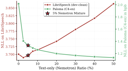
Figure below shows the impact of adding Nemotron text data on NLL for audio and text validation data:
Show full results across all metrics
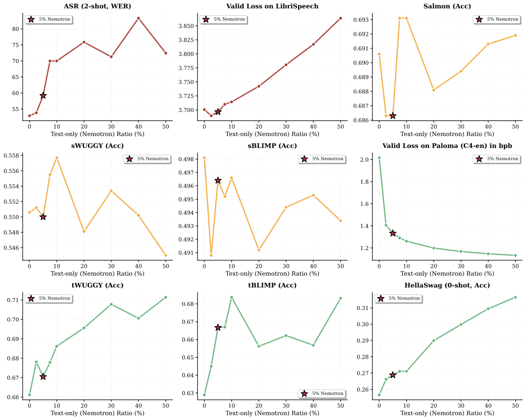
Findings
- Text knowledge improves significantly: Even a small amount of text (0% → 2.5%) causes a drastic drop in NLLtext, with continued improvement as text ratio increases. tWUGGY, tBLIMP, and HellaSwag all improve monotonically.
- Semantic/acoustic speech is unaffected: sWUGGY, sBLIMP, and Salmon show little variation across text ratios—these capabilities are robust to text inclusion.
- Cross-modal skills degrade beyond 5%: ASR and TTS plateau up to ~5% text but start degrading beyond this point.
- 5% is optimal: At 5% text, we get significant text knowledge gains with little to no degradation in audio performance. Practitioners prioritizing text/reasoning may increase this ratio at the cost of audio skills.
Decision: We fix the pre-training mixture to 5% Text (Nemotron) + 95% Speech (Yodas/Emilia) for all subsequent experiments.
Ablation on Token Composition
Goal & Motivation
We want to understand the impact of different token types on audio benchmarks. Specifically: what is the effect of (1) adding acoustic tokens to semantic tokens, and (2) interleaving text tokens alongside audio tokens?
Setup
We ablate three token configurations using a fixed budget of 3×10²⁰ FLOPs (1.7B model, 30B tokens) with Yodas as speech data (no Nemotron):
- S (Semantic-only): Only the first Mimi codebook — captures linguistic/semantic content
- S+A (Semantic+Acoustic): Up to 8 Mimi codebooks — audio-only sequences
- S+A+T (Semantic+Acoustic+Text): 8 codebooks with text transcripts interleaved at the utterance level
Results
| Tokens | Speech (Semantic) |
Speech (Acoustic) |
Text (Knowledge) |
Cross-Modal | |||
|---|---|---|---|---|---|---|---|
| sBLIMP↑ | sWUGGY↑ | Salmon↑ | tBLIMP↑ | tWUGGY↑ | ASRWER↓ | TTSWER↓ | |
| S | 58.6 | 72.1 | 67.3 | × | × | × | × |
| S+A | 50.9 | 59.0 | 70.1 | × | × | × | × |
| S+A+T | 50.4 | 58.1 | 70.4 | 67.8 | 71.6 | 18.3 | 27.1 |
S=Semantic, A=Acoustic, T=Text. × indicates the model lacks the capability to perform the task. Fixed budget: 3×10²⁰ FLOPs (1.7B model, 30B tokens).
Findings
- Semantic-only already captures rich information: Using only the first codebook already achieves 67.3% on Salmon, suggesting that the first Mimi codebook contains substantial information for audio likelihood evaluation.
- Acoustic tokens improve acoustic modeling at the cost of semantics: Adding acoustic codebooks (S→S+A) improves Salmon from 67.3% to 70.1%, but causes a clear drop in semantic understanding (sBLIMP: 58.6% → 50.9%, sWUGGY: 72.1% → 59.0%). This is a fundamental trade-off: acoustic detail competes with semantic capacity.
- Interleaving text unlocks cross-modal skills with minimal cost: Adding text tokens (S+A→S+A+T) causes only a small further drop on semantic benchmarks, no drop on acoustic benchmarks (Salmon: 70.1% → 70.4%), while unlocking ASR (18.3% WER) and TTS (27.1% WER) capabilities that are completely unavailable in audio-only configurations.
- Semantic-only models are limited in practice: While semantic-only models excel at semantic understanding (sBLIMP: 58.6%, sWUGGY: 72.1%), they lack the acoustic detail needed for high-fidelity understanding and generation.
Decision: We adopt S+A+T (Semantic+Acoustic+Text) as our token composition, accepting the semantic trade-off for broader capabilities in a unified general-purpose backbone.
IsoFLOP Study
Goal & Motivation
Scaling laws for text LLMs are well-studied (Kaplan et al., Chinchilla, Llama3, DeepSeek), yet no such analysis exists for discrete audio models (e.g., codec-based TTS models or any transformer models trained on audio tokens). Since audio tokens are typically more granular (~100 tokens/sec with 8-codebook Mimi) compared to text (~3–4 tokens/sec) at a normal speaking rate, the optimal allocation between model size and training data may differ significantly. This work conducts the first scaling law study for discrete audio models to answer:
- How should we allocate compute between model size (N) and training data (D)?
- Does the optimal point shift towards more tokens (smaller models trained longer) or larger models (trained shorter) compared to text?
- What is the optimal token-to-parameter ratio?
Setup
We conduct an IsoFLOP sweep training 64 models across seven compute budgets spanning two orders of magnitude from 3×10¹⁸ to 3×10²⁰ FLOPs. For each compute budget C, we train models of varying sizes (77M to 4.2B parameters), adjusting the number of training tokens D to satisfy C ≈ 6ND. At each budget, we identify the configuration achieving the lowest validation loss, yielding optimal pairs (N*, D*). We follow the setup of the IsoFLOP study in Relative Scaling Laws for LLMs by adapting this script.
- Models trained: 64 configurations total
- Compute range: 3×10¹⁸ to 3×10²⁰ FLOPs
- Model sizes: 77M to 4.2B parameters
- Data: 5% Nemotron + 95% Yodas/Emilia (as determined previously)
Link: 📈 WandB Log
Results
The three panels below show: (a) validation NLL vs model size N, (b) validation NLL vs training tokens D, and (c) the fitted scaling laws with extrapolation.
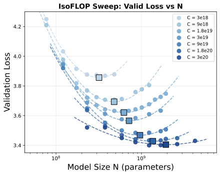
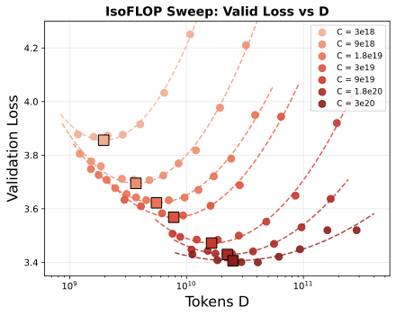
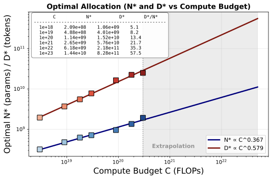
Findings
We fit power-laws N* = aN CbN and D* = aD CbD using log-linear regression to derive scaling laws for discrete audio:
- Data scales faster than model size: The optimal token count D* scales significantly faster than model size N* (0.579 vs 0.367). This means training data should grow approximately 1.6× faster than model parameters as compute budget increases.
- Consistent with low information density: These exponents differ from Chinchilla's balanced scaling (N*, D* ∝ C0.5), but align with recent text LLM findings: Llama3 reports a data exponent of 0.53, and DeepSeek finds 0.42–0.55 depending on data quality. DeepSeek interprets higher data exponents as indicative of lower information density. Our exponent (D* ∝ C0.579) fits this interpretation—discrete audio at 100 tokens/sec carries less information per token than text.
- Token-to-parameter ratio increases with scale: Unlike Chinchilla's constant ratio of ~20 tokens/parameter, the asymmetry implies the optimal ratio increases with scale: ~13 tokens/parameter at 1020 FLOPs, rising to ~58 tokens/parameter at 1023 FLOPs. This is qualitatively different from text models, where a replication attempt (Besiroglu et al.) found the ratio actually decreases with compute.
🤗 Artifacts: The collection of IsoFLOP checkpoints is available on HF: soda-research/discrete-audio-isoflop-models.
Parametric Loss Prediction
In addition to identifying compute-optimal allocations, we want to predict the expected final validation loss for models trained at larger compute budgets — including over-trained configurations where the model is trained on more data than its compute-optimal amount (e.g., our SODA-LongRun experiments in a subsequent section). To predict final validation loss, we fit the parametric equation similar to the approach in Chinchilla:
where N is the model size (parameters), D is the number of training tokens, and E represents the irreducible loss. We fit this equation on all 64 data points from our IsoFLOP sweep (not just the compute-optimal points), obtaining:
Note on derived scaling exponents. This parametric fit approach also provides an alternative derivation of scaling exponents. Using C = 6ND, the compute-optimal model size and data can be derived as N* ∝ Cβ/(α+β) and D* ∝ Cα/(α+β). Using our fitted α = 0.684 and β = 0.439, we obtain:
| N* ∝ C0.391 | (vs. C0.367 from IsoFLOP fit) |
| D* ∝ C0.609 | (vs. C0.579 from IsoFLOP fit) |
These derived exponents are reasonably close to the empirically fitted values from the IsoFLOP analysis, with both approaches showing D*/N* ≈ 1.57. This asymmetry (data scaling faster than model size) is consistent with the lower information density of discrete audio tokens compared to text.
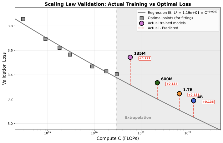
Loss predictions. The figure below shows loss predictions based on our parametric fit at different overtraining ratios K = D/D*, where K = 1 is compute-optimal and higher K indicates more overtraining (smaller model trained on more data). Grey points show IsoFLOP sweep data. Colored curves show predicted loss at K = 1 (optimal), 5, 20, and 100. Colored circles show the actual SODA models (135M, 600M, 1.7B, 4B).
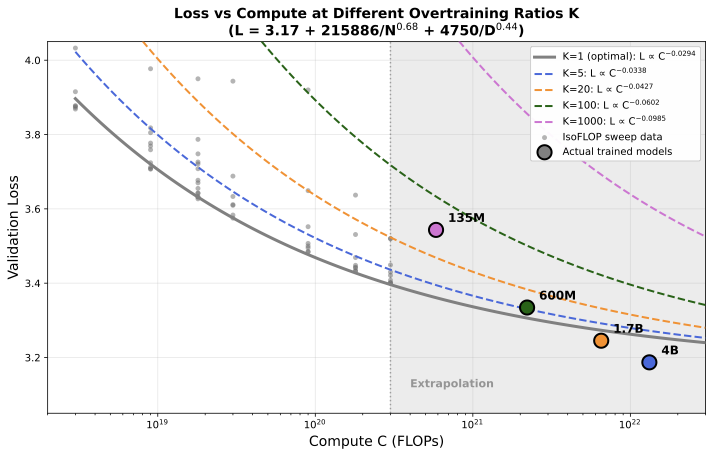
Interestingly, our longer-trained SODA models (135M–4B) in the subsequent experiment achieve losses lower than predicted by the parametric equation — even lower than the optimal (K = 1) extrapolated prediction for the 1.7B and 4B models. This systematic under-prediction when extrapolating from the IsoFLOP regime (3×10¹⁸–3×10²⁰ FLOPs) to higher compute (6×10²⁰–1.3×10²² FLOPs) could be because scaling law extrapolations diverge in the far tails of the compute distribution. The offset suggests that either scaling exponents evolve favorably at larger scales, or the irreducible loss E is lower than estimated from the smaller-scale regime. Despite these prediction challenges, downstream task performance scales reliably with validation loss (see Correlation section), making validation loss a useful proxy even when absolute loss predictions are imperfect.
Correlation between Loss and Metrics
Goal & Motivation
Before relying on validation loss (NLL) to guide scaling law analysis and future experiments, we need to verify: Is validation NLL a reliable proxy for downstream task performance in discrete audio models? If so, we can focus on minimizing NLL rather than running expensive downstream evaluations at every step.
Setup
We compute NLL on speech utterances from LibriSpeech dev-clean and analyze the correlation between NLL and downstream task performance across the 64 models from our IsoFLOP study (varying sizes and compute budgets).
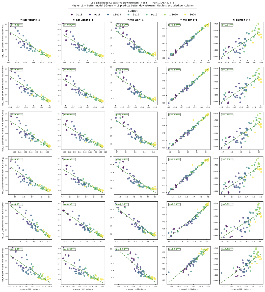
Our interleaved format admits multiple ways to compute NLL. We compare six variants:
- NLL_1: All tokens from audio+text data
- NLL_2: All audio tokens from text+audio data
- NLL_3: Semantic tokens from text+audio data
- NLL_4: Audio tokens from audio-only data
- NLL_5: Text tokens from audio+text data
- NLL_6: Text tokens from text-only data
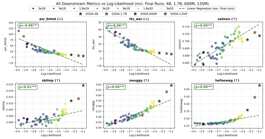
Results
The figure below shows validation NLL (audio+text) versus downstream task performance. Circular points are the 64 IsoFLOP models; star-shaped points are the final SODA runs at larger scale. Regression lines are fitted on the 64 IsoFLOP models only.
Show full results across all NLL variants (Figures)
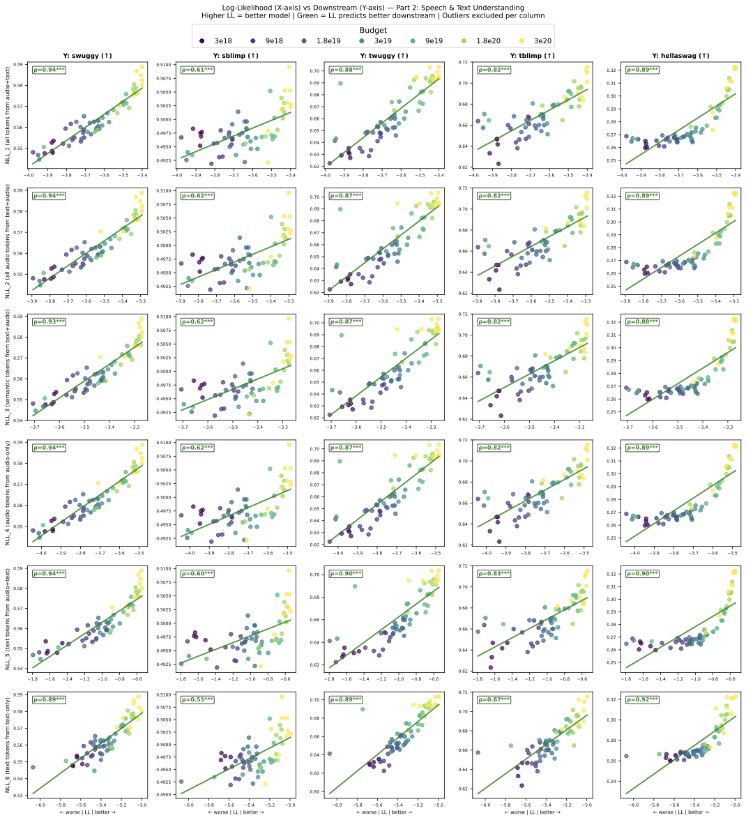
Show NLL metric comparison table (Spearman correlations)
| NLL | ASR-0 | ASR-2 | TTS-W | TTS-S | Sal. | sWUG | sBLI | tWUG | tBLI | Hella | Avg-Sp | Avg-Tx |
|---|---|---|---|---|---|---|---|---|---|---|---|---|
| NLL_1 | 0.959 | 0.967 | 0.955 | 0.989 | 0.841 | 0.941 | 0.614 | 0.879 | 0.824 | 0.887 | 0.895 | 0.864 |
| NLL_2 | 0.956 | 0.962 | 0.953 | 0.986 | 0.842 | 0.936 | 0.621 | 0.874 | 0.821 | 0.887 | 0.894 | 0.861 |
| NLL_3 | 0.954 | 0.959 | 0.952 | 0.985 | 0.842 | 0.929 | 0.620 | 0.866 | 0.819 | 0.884 | 0.892 | 0.856 |
| NLL_4 | 0.959 | 0.965 | 0.952 | 0.987 | 0.845 | 0.937 | 0.623 | 0.871 | 0.819 | 0.886 | 0.896 | 0.859 |
| NLL_5 | 0.962 | 0.961 | 0.960 | 0.986 | 0.820 | 0.944 | 0.602 | 0.899 | 0.827 | 0.904 | 0.891 | 0.877 |
| NLL_6 | 0.903 | 0.908 | 0.933 | 0.949 | 0.802 | 0.892 | 0.552 | 0.891 | 0.873 | 0.917 | 0.848 | 0.894 |
Avg-Sp averages 7 speech metrics; Avg-Tx averages 3 text metrics. NLL_1 achieves the best balance between speech and text correlations.
Findings
- Cross-modal skills (ASR, TTS): NLL is highly predictive of both ASR (ρ ≈ 0.95) and TTS quality (TTS-WER: ρ ≈ 0.96, TTS-SIM: ρ = 0.99 with near-linear improvement). However, at lower loss values, improvement slows—most results from the highest compute budget (3×10²⁰ FLOPs) fall below the regression line.
- Semantic/acoustic understanding (Salmon, sBLIMP, sWUGGY): Improvement is slow: as NLL decreases from 4.0 to 3.4, Salmon improves from 68.5% to 70.5% and sWUGGY from 54% to 58%. Salmon shows early signs of saturation at the highest compute budget. sBLIMP remains near pre-emergence (49.3% to 50.0%, near the 50% random baseline).
- Text knowledge (tBLIMP, tWUGGY, HellaSwag): NLL correlates strongly (ρ > 0.8) and improvement is more pronounced: tWUGGY improves from 62% to 69% and tBLIMP from 64% to 70% as NLL drops from 4.0 to 3.4. HellaSwag (ρ = 0.89) shows an emergence pattern: no improvement from NLL 4.0 to 3.6, then rapid increase from 25% to 32%.
- Choice of NLL metric: All NLL variants show similar correlations with downstream tasks. We select NLL on all tokens from audio+text data (NLL_1) as the primary metric because it achieves the best balance between speech (Avg-Sp = 0.895) and text (Avg-Tx = 0.864) correlations.
- Extrapolation holds at scale: The final SODA runs (trained at higher compute budgets) largely follow the extrapolated regression lines, confirming NLL as a reliable proxy even beyond the IsoFLOP regime.
SODA-LongRun
Goal & Motivation
This is the culmination of all previous experiments. Having established (1) the optimal speech data mixture (Yodas + Emilia), (2) the optimal text ratio (5% Nemotron), (3) scaling laws for discrete audio, and (4) NLL as a reliable proxy metric, we now scale up to train the final SODA (Scaling Open Discrete Audio) models ranging from 135M to 4B parameters. The key questions are:
- Do our design choices from earlier experiments generalize to larger scale?
- Does performance improve with scale across all capability types?
- How does SODA compare to existing spoken language models?
Setup & Over-Training
Training data: Following our recipe — 5% Nemotron (text-only) + 43.4% Emilia + 51.6% Yodas2 (ratio between Emilia and Yodas determined by their respective sizes). This yields ~125B + 125B = 250B tokens of interleaved speech data (audio-first and text-first formats), for a total of 500B tokens (~4 epochs). Prior work shows repeated data remains effective up to 4 epochs for LLM pre-training.
Model sizes and over-training: We train models at 135M, 600M, 1.7B, and 4B parameters, all on 500B tokens. While our scaling laws define compute-optimal token counts, inference usage favors models trained beyond D* — especially given that our 100 tokens/sec rate can make larger models slow at inference.
| Model | Parameters | Tokens | Over-training factor | Comparable to |
|---|---|---|---|---|
| SODA-135M | 135M | 500B | ~940× | — |
| SODA-600M | 600M | 500B | ~90× | Llama3 |
| SODA-1.7B | 1.7B | 500B | ~18× | Llama2 |
| SODA-4B | 4B | 500B | ~4.5× | Near compute-optimal |
Training the 4B model on 500B tokens reaches 1.3×10²² FLOPs (~1 week on v5p-256 TPU).
Experiment Script: exp1699_marin_audio_all.pyLink: 📈 WandB Log
Results
Main comparison table — SODA against existing spoken language models. SODA is the only model with capabilities across all skills, serving as a unified backbone.
| Model | Speech (Semantic) |
Speech (Acoustic) |
Text (Knowledge) |
Cross-Modal | |||||
|---|---|---|---|---|---|---|---|---|---|
| sBLIMP↑ | sWUGGY↑ | Salmon↑ | tBLIMP↑ | tWUGGY↑ | HellaS↑ | ASR↓ | TTSWER↓ | TTSSIM↑ | |
| Existing Models | |||||||||
| TWIST-7B | 59.0 | 73.9 | 61.6 | × | × | × | × | × | × |
| SpiritLM-base-7B | 58.3 | 69.0 | 57.2 | 73.3 | 80.3 | — | ~22† | ~40† | ~0.05‡ |
| SpiritLM-Expr-7B | 54.2 | 65.0 | 67.1 | 73.6 | 75.8 | — | ~38† | ~50† | ~0.10‡ |
| Llama-Mimi-1.3B | 54.3 | 68.7 | 73.6 | × | × | × | × | × | × |
| Llama-Mimi-8B | 55.1 | 68.8 | 73.2 | × | × | × | × | × | × |
| Our Models (Preliminary) | |||||||||
| SODA-prelim-600M | 50.9 | 57.8 | 69.4 | 69.0 | 71.3 | 26.2 | 22.0 | 9.2 | 0.516 |
| SODA-LongRun (Final) | |||||||||
| SODA-base-135M | 50.1 | 56.3 | 70.0 | 67.4 | 70.7 | 28.7 | 28.1 | 11.2 | 0.500 |
| SODA-base-600M | 51.2 | 58.9 | 70.1 | 70.7 | 73.1 | 35.8 | 10.2 | 7.6 | 0.555 |
| SODA-base-1.7B | 51.4 | 60.6 | 70.6 | 70.3 | 74.7 | 44.5 | 7.0 | 6.9 | 0.560 |
| SODA-base-4B | 52.4 | 61.8 | 70.4 | 71.3 | 74.8 | 52.6 | 5.0 | 6.1 | 0.560 |
× = model lacks the capability. — = not reported (HellaSwag contamination in Llama2 pre-training which SpiritLM is based on). †SpiritLM uses 10-shot eval on LibriSpeech-clean for ASR/TTS; ours is 0-shot with TTS on seed-tts-eval. ‡TTS-SIM reproduced — semantic-only tokens cannot preserve voice.
Show scaling law validation with IsoFLOP predictions
Findings
1. Do our design choices help?
Comparing SODA-base-600M to SODA-prelim-600M (both 600M, 500B tokens) validates that our design choices (English-only data, Yodas+Emilia mixture, 5% Nemotron) yield measurable improvements across all metrics:
- ASR-WER: 22.0% → 10.2% (dramatic improvement)
- TTS-WER: 9.2% → 7.6%
- TTS-SIM: 0.516 → 0.555
- sWUGGY: 57.8% → 58.9%
- tWUGGY: 71.3% → 73.1%
- HellaSwag: 26.2% → 35.8%
2. Does performance improve with scale?
We examine how downstream tasks scale, connecting to our NLL correlation analysis (see Correlation section and its figures):
- Cross-modal (ASR, TTS): ASR-WER drops dramatically from 28.1% (135M) to 5.0% (4B). TTS follows a similar pattern. However, final-run points fall above the NLL regression line, indicating diminishing returns at scale — consistent with the early saturation signs we observed in the IsoFLOP correlation analysis. SODA makes an excellent ASR/TTS backbone.
- Acoustic understanding (Salmon): Salmon saturates around 70% across all sizes (70.0% at 135M → 70.4% at 4B). This suggests acoustic ability is bounded by tokenization and/or data quality rather than model capacity. Nevertheless, this still outperforms semantic-only models (SpiritLM: 57.2–67.1%).
- Semantic understanding (sWUGGY, sBLIMP): Shows emergence — sWUGGY improves from 56.3% (135M) to 61.8% (4B), and sBLIMP from 50.1% to 52.4%. Final runs fall above the NLL regression line, suggesting accelerating gains. While still below semantic-only models like SpiritLM (likely due to content jumping between utterance chunks), the trend is encouraging.
- Text knowledge (HellaSwag): Exhibits the strongest emergence — HellaSwag accuracy jumps from 28.7% (135M) to 52.6% (4B), with final-run points appearing far above the NLL regression line. This exponential gain validates the 5% Nemotron inclusion and shows the model is learning genuine text knowledge.
3. How does SODA compare to others?
- vs TWIST (semantic-only, speech-only): TWIST-7B achieves strong semantic scores (sBLIMP: 59.0, sWUGGY: 73.9) but lacks text knowledge and cross-modal skills entirely. SODA trades some semantic performance for a vastly richer capability set.
- vs SpiritLM (semantic-only, warm-started from Llama2): SpiritLM leverages Llama2's text knowledge (tWUGGY: 80.3%), but its semantic-only tokenization limits acoustic modeling (Salmon: 57.2%) and prevents voice preservation (TTS-SIM: ~0.05). SODA's multi-codebook approach enables genuine voice quality at the cost of lower semantic scores.
- vs Llama-Mimi (semantic+acoustic, audio-only): Llama-Mimi achieves the highest Salmon (73.6%) by modeling audio-only sequences, but completely lacks cross-modal skills — no ASR, no TTS, no text knowledge. SODA's utterance-level interleaving makes it a more general-purpose foundation.
Key takeaway: SODA is the only model with capabilities across all skills — speech understanding, acoustic quality, text knowledge, and cross-modal ASR/TTS — making it a unified foundation for spoken language modeling.
🤗 Artifacts: The model checkpoints for SODA-base on HF: soda-research/soda-models.
Warm-start vs Cold-start
Goal & Motivation
Many discrete audio models (e.g., TWIST, CSM, SpiritLM) initialize from pre-trained text LLMs. Does this warm-start strategy benefit over training from scratch (cold-start)? Specifically, what skills does warm-starting improve or not improve?
Setup
We compare warm-start (initialized from Qwen3-0.6B/1.7B-base) versus cold-start (random initialization) at 600M and 1.7B scales, both trained on 500B tokens (same data and recipe as SODA-LongRun).
- Cold-start: Random initialization, standard training
- Warm-start: Initialized from Qwen3 text LLM weights (audio token embeddings randomly initialized)
- Scales: 600M and 1.7B parameters
- Budget: 500B tokens each (~4 epochs)
Link: 📈 WandB Log (same group as SODA-LongRun)
Results
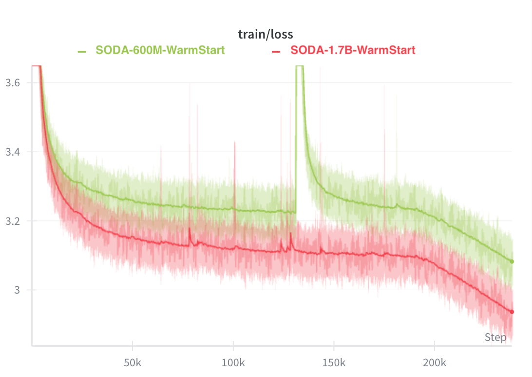
Training Loss Stability
A key observation: warm-start exhibits instability with unpredictable loss spikes, while cold-start shows smooth improvement throughout.
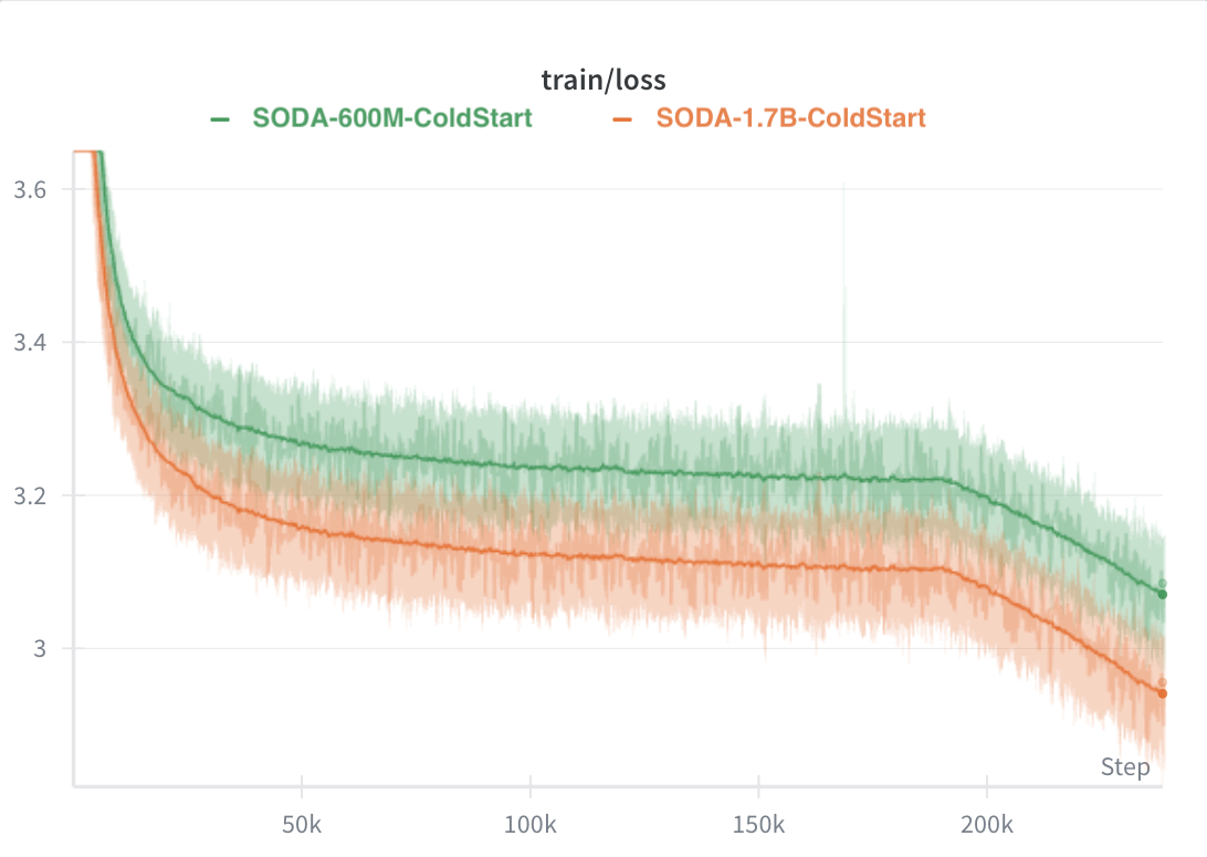
Note: With limited compute budget, we train only one run per configuration. Better regularization or different hyperparameters could potentially stabilize warm-start training.
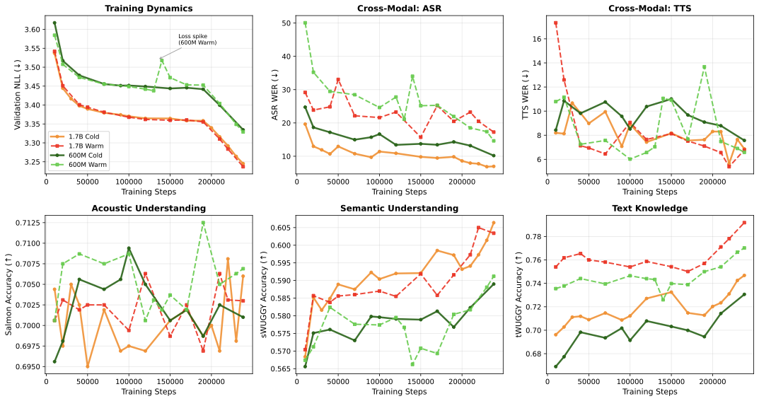
Training Trajectories
Full training trajectories comparing warm-start vs cold-start across all metrics:
Final Evaluation
| Model | Speech (Semantic) |
Speech (Acoustic) |
Text (Knowledge) |
Cross-Modal | |||||
|---|---|---|---|---|---|---|---|---|---|
| sBLIMP↑ | sWUGGY↑ | Salmon↑ | tBLIMP↑ | tWUGGY↑ | HellaS↑ | ASR↓ | TTSWER↓ | TTSSIM↑ | |
| 600M Scale | |||||||||
| SODA-600M (cold-start) | 51.2 | 58.9 | 70.1 | 70.7 | 73.1 | 35.8 | 10.2 | 7.6 | 0.555 |
| SODA-600M (warm-start) | 51.1 | 59.1 | 70.7 | 70.8 | 77.0 | 36.3 | 14.6 | 6.6 | 0.559 |
| 1.7B Scale | |||||||||
| SODA-1.7B (cold-start) | 51.4 | 60.6 | 70.6 | 70.3 | 74.7 | 44.5 | 7.0 | 6.9 | 0.560 |
| SODA-1.7B (warm-start) | 51.8 | 60.3 | 70.3 | 71.0 | 79.2 | 47.1 | 17.3 | 6.8 | 0.557 |
Findings
- Training stability: Warm-start exhibits instability with unpredictable loss spikes (including a large spike at 135K steps in the 600M run, where ASR degrades from 21% to 34%). Cold-start shows smooth improvement throughout.
- Cross-modal skills (ASR): Cold-start outperforms warm-start on ASR from the earliest checkpoint. At 1.7B, cold-start achieves 19.7% vs 29.2% WER at 10K steps, widening to 7.0% vs 17.3% at completion. This suggests warm-start may interfere with learning audio→text mappings.
- Cross-modal skills (TTS): Cold-start is initially better, but warm-start catches up. Both achieve comparable TTS quality at completion (~6.5–7.5% WER, ~0.56 SIM).
- Speech understanding (Salmon, sWUGGY): Similar trajectories regardless of initialization (~70% Salmon, ~60% sWUGGY), suggesting these audio skills are learned fresh regardless of starting point. This is consistent with SpiritLM's findings (their Table 6).
- Text knowledge (tWUGGY, HellaSwag): Warm-start begins with a substantial advantage (at 10K steps: tWUGGY 75.4% vs 69.6%, HellaSwag 40.5% vs 29.9%). Critically, cold-start never catches up even after 500B tokens (final tWUGGY: 74.7% vs 79.2%; HellaSwag: 44.5% vs 47.1%), indicating text knowledge from LLM pre-training is not fully recoverable through audio-centric training.
Recommendation: We recommend cold-start as the default recipe for general audio capabilities, given the training instability and ASR degradation from warm-starting. However, for applications where complex reasoning or text knowledge is critical, the persistent text-knowledge advantage of warm-start may outweigh these downsides. A hybrid approach (cold-start pre-training followed by text-enriched fine-tuning) is an interesting future direction.
🤗 Artifacts: The model checkpoints for SODA-warmstart on HF: soda-research/soda-warm-start-qwen3-based-models.
Open Questions & Future Directions
While this work establishes a scaling law and training recipes for discrete audio models, there remain some interesting open questions for future work.
1. Where is the Emergence?
Unlike text LLMs which exhibit emergent capabilities at scale (e.g., unseen skills like arithmetic, reasoning, in-context learning), this work did not observe strong emergent speech or audio capabilities from pre-training alone. Our models require fine-tuning to unlock their full potential, similar to the BERT/BART/GPT-2 era in NLP.
- Question: Does audio require significantly more scale (parameters or data) than text to show emergence?
- Question: Is next-token prediction on flattened sequences sufficient for hierarchical audio structures, or do we need different objectives?
- Direction: Investigating audio few-shot learning to see if capabilities can be prompted rather than fine-tuned.
2. Resolving the Semantic-Acoustic Trade-off
Our results show a trade-off between what is said (semantic) and how it is said (acoustic). Adding acoustic tokens improves fidelity but degrades semantic understanding (sBLIMP/sWUGGY drop).
- Question: Can we decouple these trade-offs using multi-module/stream architectures or curriculum learning (e.g., start semantic, fade in acoustic)?
- Direction: Exploring RVQ-weighted loss functions (weighting earlier codebooks higher) to force the model to prioritize semantic content (codebook 0) before optimizing fine acoustic details.
3. Unexplored Design Choices
We selected the Mimi tokenizer and a specific interleaving pattern, but the design space is vast.
- Alternative Tokenizers: Would other tokenizers perform better or yield different patterns?
- Sampling Rates: We used a fixed frame rate. What is the optimal token-to-second ratio for efficiency vs fidelity?
- Disentanglement: Can we design tokenizers that explicitly disentangle content/semantics from speaker identity/prosody?
4. Data Scaling Laws for Audio
We found that optimal data size scales 1.6× faster than model size (D* ∝ N*1.6), consistent with the hypothesis that discrete audio tokens have lower information density (lower entropy) than text tokens.
- Question: Does this exponent hold for larger models, or does it saturate? Or general audio data (beyond just speech)?
- Question: How does this ratio change with better audio tokenizers (higher compression)?
5. Path to LLM-level Knowledge
An overarching question is whether training on audio data (even with interleaved transcripts) can ever reach the reasoning and world knowledge capabilities of text-trained LLMs.
- Question: Is there a theoretical limit to knowledge acquisition from speech due to the lower information density or the conversational nature of most speech data?
- Question: Can we bridge the gap by simply scaling up, or is a fundamental architectural change (e.g., warmer starting points, hybrid objectives) required?